Mapping Roasting Plans Between Different Machines

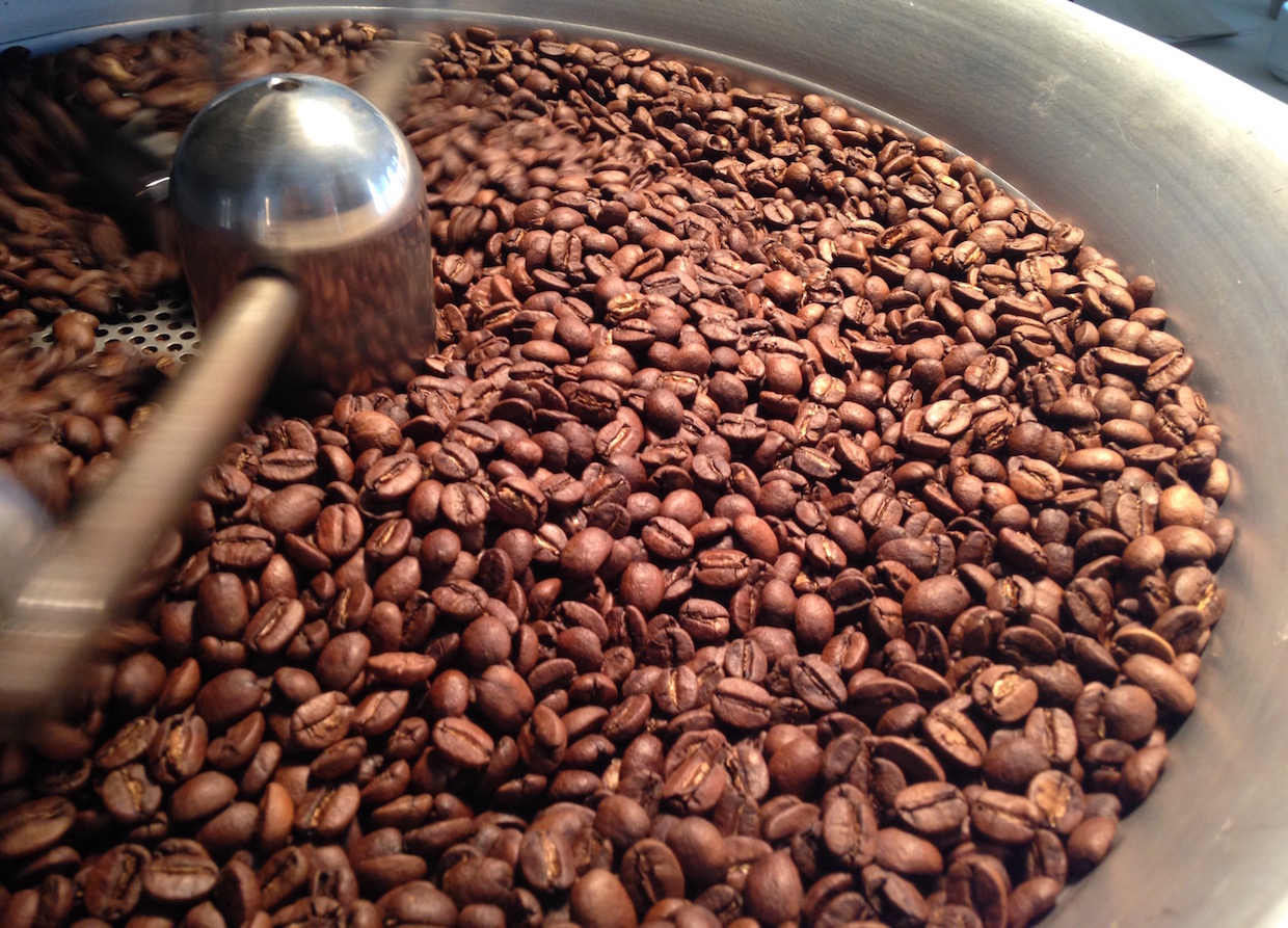
Daily Coffee News photo.

These measurements may differ from what you see on your machine.

This is a disclaimer commonly heard in coffee roasting classes.

Why? There are several reasons, actually. Different technologies are in use for measuring the temperature of coffee seeds in the machine; probe placement varies; and the differences in the roasting vessel and how air moves through it will also have an impact on what temperature values are measured when roasting coffee.

In general, this isn’t a problem for professional coffee roasters. You learn the characteristics of the machine you’re working on, and as long as that’s consistent from one batch to the next, you can build a useful body of experience to roast on that machine.

In 2012 I installed a Diedrich IR-1 lab roaster in my shop. Talking with people from Diedrich Manufacturing, I learned that one of the design goals for this machine was to allow roasters to develop their roasting plans on this smaller machine and have the ability to transfer that roasting plan to a larger machine and obtain the same results in the cup.

Perhaps that worked with roasters built around the same time, but my Diedrich IR-12 is 12 years older than my IR-1. It quickly became apparent that the longer, thinner thermocouple in my IR-12 produced different measurements than the shorter, thicker thermocouple in my IR-1, but both machines were self-consistent from batch to batch.

Since I had written a program called Typica to handle data acquisition at these machines, it seemed to me that if I could characterize those differences, it would be possible to have the software take measurements from the IR-1 and pass those through a mapping function that would produce the values that I would have measured if I were roasting on the IR-12.

Understanding how to construct these mapping functions makes it easier to apply knowledge acquired at one roasting machine to the process of roasting on a different machine. The characteristics of these mapping functions have implications for the general validity of certain analytical techniques.

Creating a Mapping Function

A function is a mathematical relationship that takes any input in its domain and produces exactly one solution. If you were to graph a function on a single variable (x) with a solution (y), you would find that for every x there is exactly one solution y. For example, when roasting a coffee, at any moment in time (x), our seed temperature probe reads exactly one temperature (y).

In this application, we’re interested in taking the temperature values measured on one roasting machine (x) and producing the temperature values that would have been measured if we were roasting that coffee on a different machine (y). If roasting plans are portable between the two machines, we would expect to derive the equation y=x.

The first step is to make some observations. Pick a fresh, high-density coffee with good physical uniformity that will show obvious changes in color and produce clear, tight cracking sounds. Roast a batch at a similar proportion of capacity on each machine, attempting to roast to the same ending color in about the same amount of time on each machine.

While doing this, observe the measured temperatures when the seeds change in color from green to yellow, from yellow to brown, and when first and second cracks can be heard. The nice thing about these points is that the changes are easy to observe and they occur at consistent temperatures for a given coffee. If you’re interested in dark roasts it can be useful to have one more pair of equivalent points beyond second crack.

That last point is more difficult to determine because it doesn’t correspond to an obvious physical change. Time and color can be used for an initial guess but this choice should be verified or rejected based on equivalence of flavor in the cup.

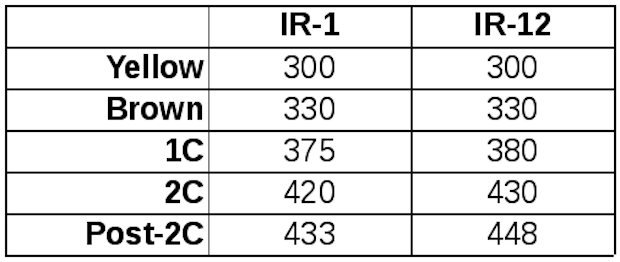
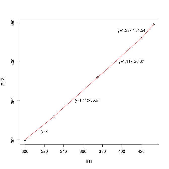
In this case, temperature measurements at the first two observation points are identical, but as the roasts progress the difference in measured values increases. This means that our mapping function must be non-linear. This is easy to see graphically by placing the points on a graph and using linear spline interpolation to connect the dots with line segments, as in the example graph below. When performing this kind of interpolation, our observation points are called knots.

Remembering the formula to represent a line, y=mx+b, m is the slope of the line. In this example we can see that thermocouples on the two machines read exactly the same until reaching the color change from yellow to brown. After this, the slope of the line increases slightly, but that slope is the same for both the segment ending at first crack and for the segment ending at 2nd crack. After 2nd crack, the slope increases again.

It’s important to note that these sharp changes in slope are likely an approximation of an underlying curve, but this curve only bends slightly in the range of values we’re interested in, so this approximation is close enough that it isn’t worth the effort of deriving that underlying curve. If it turns out that there’s an area where the error introduced by this approximation is large enough to produce differences that can be detected in the cup, this can be fixed by adding another knot, or observation point, to the linear spline.

A nice side effect of the choice of linear splines is that with two knots it’s possible to model a constant offset simply by having our y value on both points at a fixed distance from the x value. Similarly, a linear relation can be modeled by providing two points along that line. Regardless of whether we’re modeling an underlying curve or something simpler, to cover temperature measurements lower than the first knot and higher than the last knot, we can just extrapolate from each end.

Verification

How far does getting equivalent temperature measurements go toward the goal of being able to create a roasting plan on one machine and getting the same results in the cup on a different machine? To find out, we can take existing roasting plans from the larger roaster, recreate these on the smaller roaster, and compare cupping results. It’s best to try this across a broad range of final roast levels and with different roasting styles to either maximize confidence that this can be used for future product development or to determine conditions where this doesn’t work.

When comparing results in the cup, it’s best to do this with a blind triangulation cupping or something similar with more cups, such as a 2-of-5 test. Cuppers should first try to identify which cups are different in each set and then judge how significant that difference is. If people cannot reliably determine which cups are different, we can be confident that product development work can be done with the smaller roaster with less coffee.

If subtle differences are consistently detected, this might still be considered good enough or you might use those sensory differences as clues to make small adjustments to the knots and try again. Another possible result is that some roasting styles will match very well while others will have differences in the cup. That generally indicates that the two machines have significant design differences that are impacting flavor in the cup. In that case it can still be useful to start product development work with an approach that does map well to the other machine and adjust roasting plans into non-portable styles only when needed for a specific desired sensory result.

In this example, the results were good enough without making any changes to this initial mapping function, and after five years of successfully using the smaller machine for product development work, I think it’s safe to conclude that this has worked better than I could have expected for these two machines.

These results come from two machines that were designed to have very similar heat transfer characteristics. Since then, I’ve repeated this exercise with other machines as I’ve traveled to different events and taught roasting classes on machines from several different manufacturers. By understanding how measured values at the roaster I was using compared with what I see in my shop, it’s easier to relate those experiences to students. The specific mappings with different machines vary, but in my experience the functions are always non-linear.

Implications for Rate of Change Data Analysis

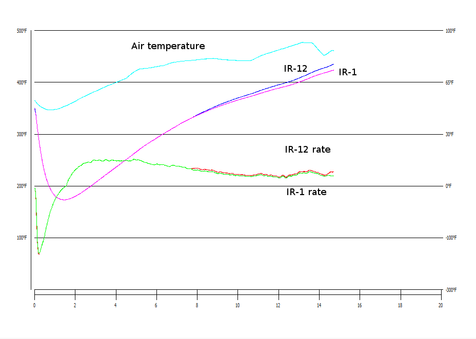
One of the most significant features made possible by modern data acquisition tools is real time calculation, display, and graphing of the rate of change of the seed temperature. Having that information available at a glance makes it easier to read ahead while attempting to match a roasting plan, and it helps roasters roast coffee more consistently from batch to batch.

Many roasters have attempted to connect sensory experiences in the cup with this rate of change data. This includes establishing upper and lower bounds on acceptable rates of change or connecting how the rate of change changes at certain parts of the roast to specific sensory differences.

While these observations might be valid for a given machine and this may be useful knowledge within a company, a consequence of the findings here is that any such analysis of rate of change data is inherently non-portable to different machines unless supporting data is presented with enough detail for roasters to construct their own mapping functions to their own machines. Failure to understand this has resulted in too many discussions supposedly about coffee roasting that are really about an arbitrary aesthetic quality of the graph.

Since the range of measured values is different for equivalent roasts on different machines, the magnitude of the rate of change will be different as well. More subtle is that as a consequence of these mapping functions being non-linear, what looks like a descending rate of change for some part of a roast on one machine can look like a steady or even increasing rate of change on a different machine. Pretending that analysis based on rate of change data can reliably be transferred among the broad range of machines currently in use ignores the physical realities of the measurement tools in use.

Conclusion

Knowing how to create these mapping functions, understanding their general characteristics, and knowing the limits of how these can be applied among your machines provide roasters with a powerful tool for designing new roasting plans. It allows roasters to roast smaller product development test batches with confidence that the final roasting plan can be used with a larger production roaster.

While it is possible to apply these functions by hand, software that could support this kind of mapping with linear splines makes it much easier to use this technique, and having these mappings applied automatically also makes it easier for a roaster to constrain their product development test batches to roasting plans that are possible to execute on a larger machine. Understanding the implications of this mapping for rate of change data should help roasters avoid spending too much time on work based on roasting theories that were presented without adequate rigor which might not be applicable to their machines.